Pontryagin's Minimum Principle

In the previous posts, a good introduction to the field of optimization and its relevance to the domain of hybrid electric vehicles was explained. Delving deeper into this concept, we’ll be discussing another of the more popular optimization algorithms used in this field, the Pontryagin’s Minimum Principle.

Background

First formulated in 1956 by Russian mathematician, Pontryagin and his students, this theory has gained a wide following in the optimal control domain. Its roots can be traced back to the Calculus of Variations and the subsequent development of Bellman’s principle of optimality. Another similar theorem to which it is frequently compared is the Dynamic Programming based on the Hamilton-Jacobi-Bellman equation which was discussed in the previous post. A comparison between these is offered towards the end of this post.

The Principle

This theory has a single goal in mind: find the optimal trajectory for a state vector keeping in mind the required constraints and therefore find the optimal control vector for effecting this trajectory.

Mathematically, this can be expressed as in the following equations. Here, I aim to translate the existing mathematical equations to our optimization problem.

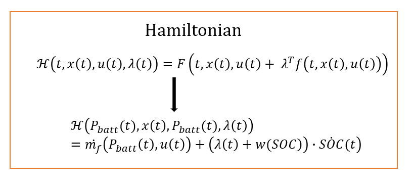
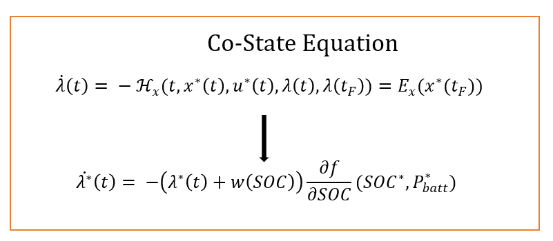
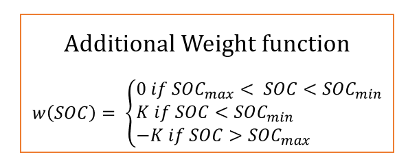
Using these equations, we can implement this algorithm. Let's have an overview of the implementation with a flowchart.

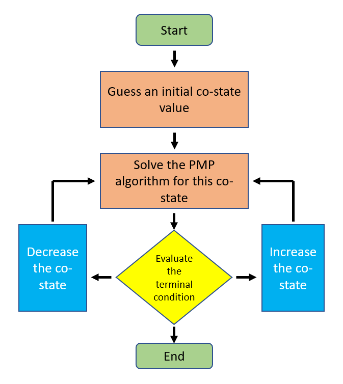
Now that we have a basic idea of the algorithm, let's take a step further and implement this control concept in Matlab. Like many other algorithms, there are numerous ways of going about this implementation. Some possibilities include use of the 'dsolve' and 'syms' commands in Matlabor probably you'll be interested in using mathematical solvers like CasADi or Yalmip to solve this problem completely. They do also have an advantage of having cross-platform support and quite good documentation. However, here we will use a simple 'nested for-loop' structure find the optimal trajectory. Los geht's !

You can find the entire code here. If you want, you can download the code here and work them with me. Of course, I have tried my level best to comment the important steps. So, the first thing to take of is the Driving cycle initialization. Here, I have used the Urban Dynamometer Driving Schedule (UDDS) cycle for my computation.

  load('UDDS_drive_cycle.mat');
  Cycle.ts =1;
  Cycle.N=length(t);
  Cycle.P_dem = P_dem';

Let's now go ahead and create the matrices for our Battery and Engine components. We also need to define some parameters for modelling these components.

%% Battery Inputs
Bat.P_max = 15; % in kW
Bat.lb_SOC = 0.3; Bat.ub_SOC = 0.8; % Upper and Lower Limits of SOC
Bat.lb_P   = 0.1*Bat.P_max; Bat.ub_P= 0.9*Bat.P_max; % Upper and Lower Limits of Power Deliverable
Bat.U_oc = 320; %in V
Bat.Q_bat = 18000; %Battery Capacity
Bat.R0_B = 0.001; % in Ohm
Bat.P_bat     = zeros(Cycle.N,1);
Bat.SOC = zeros(1,Cycle.N);
Bat.SOC(1,1) = Bat.ub_SOC;

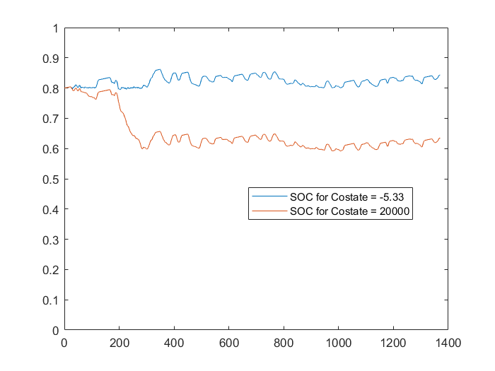
Here, we have assumed that we start our journey with 80% SOC. It would be our mission to tune the algorithm sufficiently to ensure that the SOC at the end of the journey is as close to this initial value as possible.

%% Engine Modellling
Engine.P_engine  = linspace(1,20,1000)';
Engine.P_opt_eng = zeros(Cycle.N,1);
Engine.fl_wy_en = 0.001;
Engine.P = Engine.P_engine(1,1);
Engine.eff = 0.45;

Now that the modelling is taken care of, let's start with the actual algorithm implementation. But before that, let's first intialize the costate vector and the weighting factor vector and then proceed with the implementation.

 %% PMP Implementation
 costate_p = zeros(Cycle.N,1);
 w_factor =  zeros(Cycle.N,1);
 
 SOC_1 = pontryagin(-5.33,Bat,Cycle,Engine);
 SOC_2 = pontryagin(20000,Bat,Cycle,Engine);

As you can see, we have used 2 different initial values for our costate here. This will help us appreciate the difference between the two different trajectories that our system will take under these two different conditions.

function soc = pontryagin(p0,Bat,Cycle,Engine)
costate_p(1,1) = p0;

for i = 1:Cycle.N-1
    Bat.P_bat = Cycle.P_dem(i) - Engine.P;
    if Bat.SOC(i)<=Bat.lb_SOC
       w_factor(i)=-10^8;    
    elseif Bat.SOC(i)>=Bat.ub_SOC 
       w_factor(i)=+10^8;
    else
       w_factor(i)=0;
    end    
    I_bat = (Bat.U_oc-sqrt(Bat.U_oc^2-...
       Bat.R0_B*Bat.P_bat*1000*4))/(Bat.R0_B*2); 
    Del_soc = -(Cycle.ts*I_bat)/(0.9*Bat.Q_bat);
    H = Engine.fl_wy_en*Cycle.ts*Engine.P_engine/Engine.eff +...       
       (costate_p(i)+w_factor(i))*Del_soc;
    H_min = H;
    P_eng = Engine.P;
    for j =2:length(Engine.P_engine)
       Engine.P = Engine.P_engine(j,1);
       Bat.P_bat = Cycle.P_dem(i)-Engine.P;
       I_bat = (Bat.U_oc-sqrt(Bat.U_oc^2-...
          Bat.R0_B*Bat.P_bat*1000*4))/(Bat.R0_B*2); 
       Del_soc = -(Cycle.ts*I_bat)/(0.9*Bat.Q_bat);
       H = Engine.fl_wy_en*Cycle.ts*Engine.P_engine/Engine.eff +... 
          (costate_p(i)+w_factor(i))*Del_soc;
       if H_min > H
          H_min = H;
          P_eng = Engine.P;
       end
    end
    Engine.P_opt_eng(i) = P_eng;
    Bat.P_bat(i)     = Cycle.P_dem(i)-Engine.P_opt_eng(i);
    I_bat        = (Bat.U_oc-sqrt(Bat.U_oc^2-...
      Bat.R0_B*Bat.P_bat(i)*1000*4))/(Bat.R0_B*2);
    Bat.SOC(i+1)     = Bat.SOC(i) - (Cycle.ts*I_bat/(0.9*Bat.Q_bat));
    del_p =  costate_p(i)* 1 / Bat.Q_bat * (1/(2*Bat.R0_B) -... 
      1/(4*Bat.R0_B^2) * Bat.U_oc / sqrt(Bat.U_oc^2/(4*Bat.R0_B^2) -... 
      Bat.P_bat(i)*1000/Bat.R0_B)) * 1;  
    costate_p(i+1) = del_p*Cycle.ts + costate_p(i);
 end
 soc = Bat.SOC;
 end

In following these steps, the PMP will have been implemented. Once, this code is simulated in Matlab, we can find that the SOC curves for this use case are as below.

Some important pointers of this theorem:

· Maximization of the Hamiltonian is easier than the original multi-dimensional problem, this is because in this algorithm, the optimization is worked on a pointwise basis.

· This method is computationally more efficient than the HJB-equation based Dynamic Programming algorithm.

· However, unlike the DP, the output value may not be globally optimum. This is because, the values are checked for a particular trajectory and not the entire spectrum of the possible trajectory.

· The particular trajectory on which the PMP algorithm is computed is based on the initial condition, also known as the initial costate. Therefore, there is a need for a prior calculation to determine the most accurate costate for that particular model.